

This is the fourth post in a series looking at elements of option trading and option risk management.
In the earlier posts (part 1, part 2, part 3) on this subject we defined gamma as the rate of change of delta. We argued however, that this was not a particularly intuitive definition. One alternative was to think of it of as a trader’s exposure to actual (‘realised’) volatility. If spot becomes more volatile, delta changes and gamma will help the trader estimate the magnitude of this change.
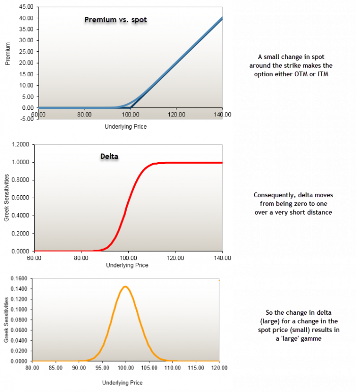
The spot – delta – gamma relationship
Here is a diagram that shows the relationship between movements in spot, delta and gamma.
One key point always is that expecting spot to be volatile is not the same as expecting an increase in implied volatility. In a Black Scholes Merton (BSM) model the two parameters are independent although admittedly they may well be related. However, there is a neat trick we can use that will link the two concepts together.
Translating volatility into a trading range
In our previous examples, we valued the option using an implied volatility of 60%. This measures the range of expected price movements over the life of the option. The input to a BSM model is a percentage per annum value irrespective of the option’s maturity. The internal maths of the model will then prorate this value based on the time to maturity. So how is this done?
The first step is to consider the number of trading days in a year. But in doing so remember that option markets do not trade at the weekend. Although subject to some debate, let us use a figure of 250. In our examples we had assumed that the option’s maturity was three months or 92 days. It might be tempting to say that the volatility expected over this period is 60% x 92 /250 or about 22%. However, the maths of option valuation work on the basis of the “square root of time” rule. There may be some debate as to how this is done but one popular method would be to dividend the volatility input (in % per annum) by the square root of the number of subperiods in 1 year. Since there are four, three month subperiods in a year this would return a value of 30% [60% / SQRT (4)]
Our example was based on a one day movement of prices so applying the same principle returns 60% / SQRT (250) = 3.80%. Note that some traders will assume 256 trading days, so the denominator has a nice round value of 16.
How would we interpret this result? If we know that the current spot price is $1,000, we expect the share to trade within an approximate range of values of +/- 4%, i.e., $960 – $1,040. When illustrating gamma in the previous posts, we looked at a + / – 10% range of values meaning actual volatility was greater than implied. Since the trader had sold the option, this was one of the reasons why they lost money.